WARNING: This post assumes you have a basic understanding of neural networks and specifically Recurrent Neural Networks (RNNs) and it assumes that you have read part 1.

Now we have a solid understading of the basics of attention mechanisms, I’m going to dive right into transformers. This post will be largely based on the original Transformers paper, Attention Is All You Need, but will also include additional intuitive explanation, technical details, and important context.

I have not yet implemented this paper, but I found this good PyTorch implementation online. I might come back to this post and add my own implementation 🙃.

I want to start by giving relevant background to the problem this paper aims to address.

Transduction in Machine Learning

Transfomers were originally created as transduction models in NLP. There are several definitions of transduction models, but the definition that seems most in line with how the paper uses it is “learning to convert one string into another”. Neural machine translation (explained in the last post) is one of many problems that a transduction model can be used for.

Problems with Previous Transduction Models

Before 2017, when Transformers were introduced, the state of the art (SOTA) in transduction problems were mostly LSTMs, GRUs, and their variants. The problems with these models is they are recursive in nature. Recurrent models require the previous hidden state in order to compute the current hidden state, meaning they are sequential. This reduces computational efficiency because it prevents parallelization within training examples, which is especially important for training with longer input sequence lengths (training on longer articles and documents).

There is a body of existing literature which achieves parallelization though the use of convolutional neural networks (CNNs), yet these models still struggle at learning dependencies between words that are far apart, because the number of operations required to relate words that are far apart increases with their distance. Transformers are the first transduction architecture that achieves parallelization within training examples (without convolutions or recurrence, by using attention for everything) and maintains a constant number of operations to relate words of any distance. As we will soon see, this allows transformers to achieve SOTA performance in transduction tasks with less training time than previous models.

Transformers Architecture Explained

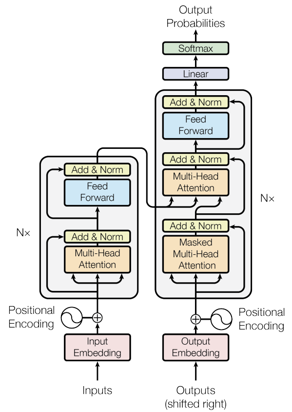
Now for the fun part! I’m going to explain transformers by going step-by-step through a forwards pass. I will frequently reference this diagram from the paper:

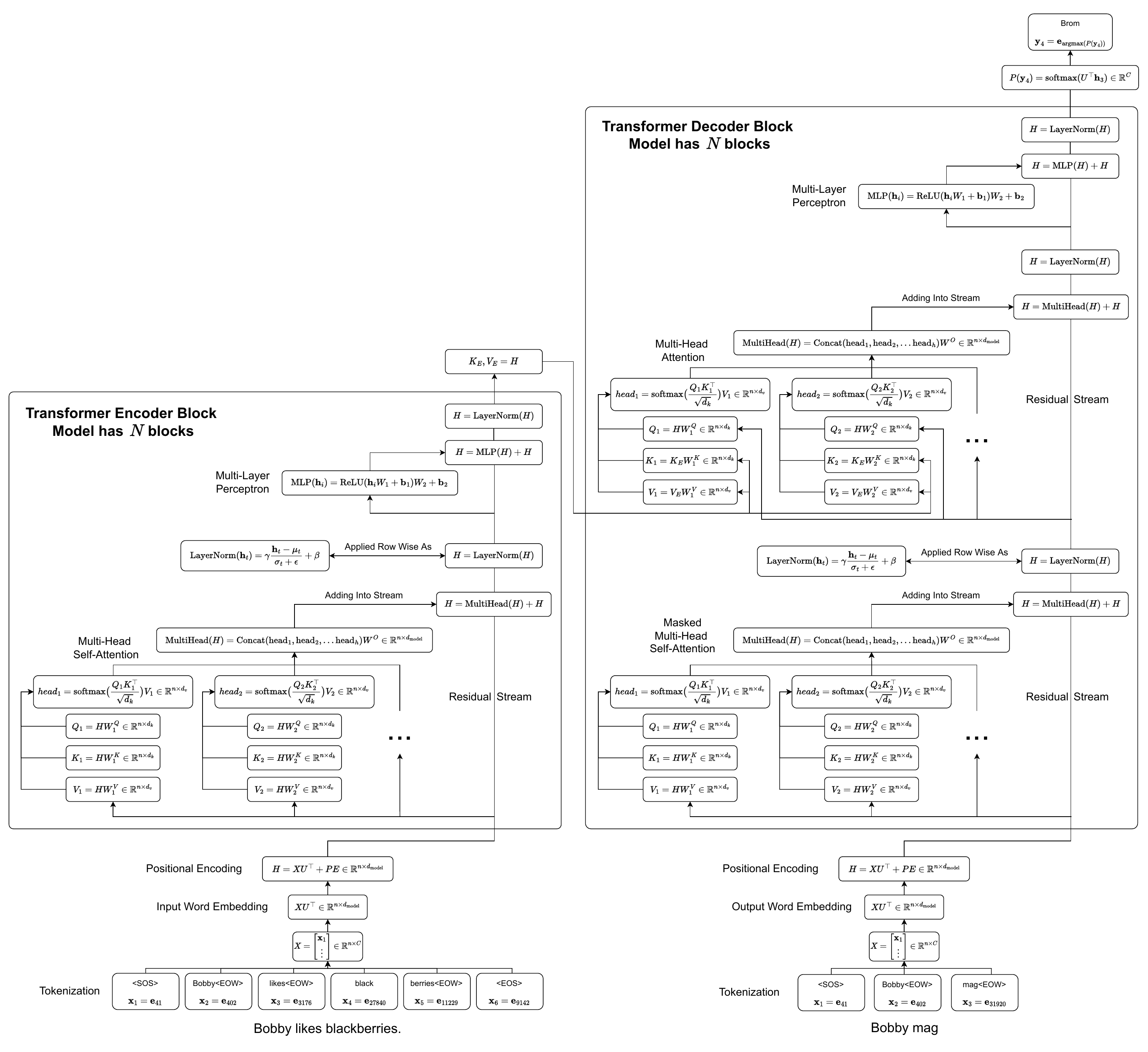
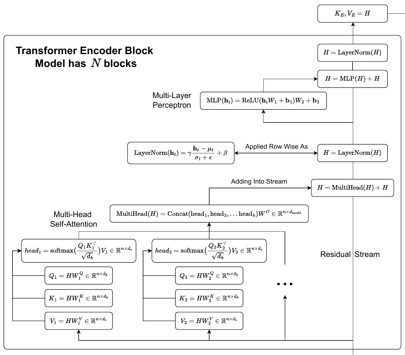
Additionally, I have created my own diagram which explains things a bit more throughly. The diagram is quite big, so I recommend going to this link to see the full pdf or opening the below image in a new tab. I have copy pasted bits of the diagram into the relevant sections, but you can also view the full diagram here:

The model resembles the encoder-decoder structure of previous transduction models (see part 1 for details).

Mathematical Notation

\(\textbf{x} \in \mathbb{R}^d\) will denote a column vector comprising of \(x_1, x_2, \ldots, x_d\). I will often use a data matrix denoted as \(X \in \mathbb{R}^{n \times d}\), where the \(i\)th row corresponds to the row vector \(\textbf{x}_i^\top \in \mathbb{R}^d\). Therefore, by writing \(\textbf{x}_i\) I am refering to a column vector of the \(i\)th row of \(X\).

\(X \in \mathbb{R}^{n \times C}\) and the corresponding \(\textbf{x}_i\) vectors will represent the input words, \(H \in \mathbb{R}^{n \times d_{\text{model}}}\) and the corresponding \(\textbf{h}_i\) vectors will represent the hidden state, and \(\textbf{y}_i \in \mathbb{R}^C\) will represent the output logits for the \(i\)th output word.

Pre Encoder

I'm going to use these green blockquotes to show a running example for the embedding and unembedding of translating the sentence "Bobby likes blackberries." to German, "Bobby mag Brombeeren."

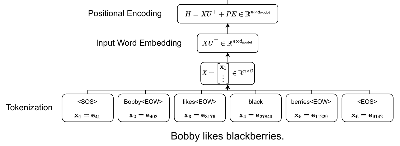
The input to our model is the text "Bobby likes blackberries."

Tokenization

The first challenge is to convert the input string to a meaningful representation that the model can work with. The cannonical way to do this is to assign one hot vectors to your input corpus. The only question is what unit of your input vocabulary should you assign one hot vectors to? Should each character have it’s own vector? Should each word have it’s own vector?

The original transformers paper, along with many other modern implementations, uses byte-pair encoding (BPE) to create subword tokens that can be assigned to one hot vectors (37000 tokens for English to German in the paper). It allows for common words to have their own representation, but breaks rare words into multiple subtokens in order to include all words in the corpus without an incredibly large vocabulary. Here is how BPE works (visit this page for a more detailed walkthrough of this algorithm):

1. Split up the entire corpus into characters and add a special start of sentence token <SOS>, end of word token <EOW>, and end of sentence token <EOS>. This is the initial token list.
2. Count all token pairs and replace the individual tokens of the most common pair with the pair itself.
3. Repeat step 2 until the desired vocabulary size, \(C\), is reached.

Now that we have split up the input sentence into meaningful tokens, we can create one hot vectors from these tokens. I will be using the following notation to represent one hot vectors: $\textbf{e}_i \in \mathbb{R}^C$, where $\textbf{e}_i$ is the $i$th standard basis column vector. In other words, $\textbf{e}_i$ represents a one hot vector where the value corresponding to the $i$th dimension is 1 and the rest are 0.

After tokenization, our input sentence "Bobby likes blackberries." is turned into the following list of tokens ["<SOS>", "Bobby<EOW>", "likes<EOW>", "black", "berries<EOW>", "<EOS>"] using BPE with vocabulary size $C = 37000$. Now we can vectorize this list to get $\begin{bmatrix} \textbf{e}_{41}^\top \\ \vdots \end{bmatrix} = \begin{bmatrix} \textbf{x}_1^\top \\ \vdots \end{bmatrix} = X \in \mathbb{R}^{n \times C}$, where $\textbf{x}_i$ is the one hot vector for the $i$th input word and $n$ is called the context size. More details on the value of $n$ can be found in the decoder section.

(Please note that the output tokens are from BPE and your one hot vectors depend on your input and I'm just arbitrarily choosing plausible values.)

Word Embeddings

But these one hot input vectors are still very high dimensional. Luckily, we can embbed these vectors into a lower dimensional vector space that is easier for the model to work with. To do this, the original transformers paper uses weight sharing of the input embeddings, output embeddings, and unembedding to get the logits, similar to what was done by Press et al. (see the paper for more details, I will just give a brief explanation).

A word embedding matrix \(U \in \mathbb{R}^{d_{\text{model}} \times C}\) (\(d_{\text{model}}\) is just the dimension of many word representations in the model, it is \(512\) in the original transformers paper) is used to convert \(\textbf{x}_i\) into a lower dimensional vector \(U \textbf{x}_i \in \mathbb{R}^{d_{\text{model}}}\) that matches the model size and represents the properties of the input word. We will use the same matrix \(U\) to unembed our hidden state to get the logits (see post decoder section). We train \(U\) along with the rest of our network (no pretrained word embeddings used).

Now we can take our list $\begin{bmatrix} \textbf{x}_1^\top \\ \vdots \end{bmatrix} = X$ of token one hot vectors, and compute the word embeddings $\begin{bmatrix} (U \textbf{x}_1)^\top \\ \vdots \end{bmatrix} = X U^\top \in \mathbb{R}^{n \times d_{\text{model}}}$.

Positional Encodings

Because transformers don’t have any sort of recurrence or convolutions, the model has no way of understanding the order of the inputs. The model needs some form of positional encoding of the input tokens. In the original transformers paper, these encodings were explicitly given and not learned (empirical evidence suggests learned embeddings didn’t perform better in general and even performed worse for input sequences longer than the ones in the training data).

Where \(pos\) is the position of the token and \(i\) is a dimension in that token’s embedding. This is what the encodings partially look like (image taken from the illustrated transformer).

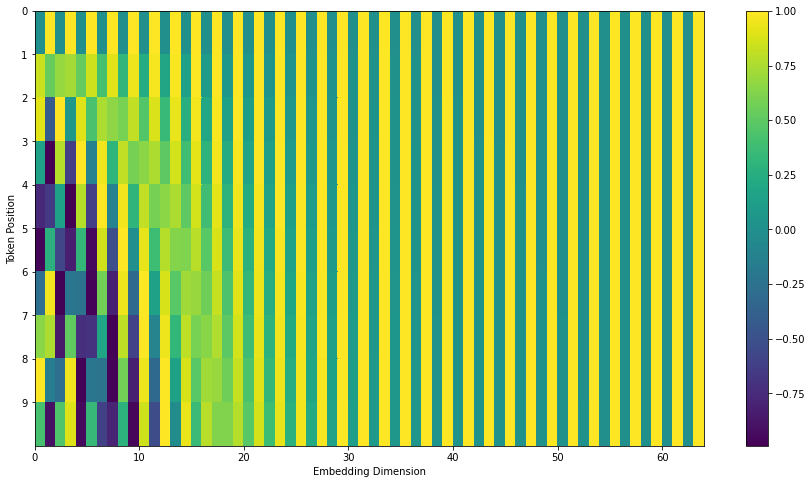
The authors hypothesized that these positional encodings would allow the model to easily learn to attend by relative positions, since for any fixed offset \(k\), \(PE_{pos+k}\) can be represented as a linear function of \(PE_{pos}\).

These positional encodings get summed with the original embeddings to create the input into the transformer encoder. I’m going to use \(H \in \mathbb{R}^{n \times d_{\text{model}}}\) to indicate hidden state of the model (note that the dimension of the hidden state never changes in any of the transformer layers).

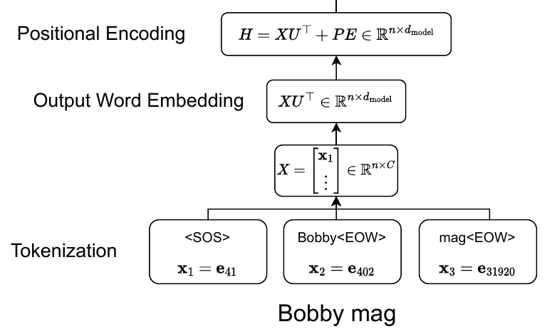
We can represent our input sentence as $H = X U^\top + PE \in \mathbb{R}^{n \times d_{\text{model}}}$, where we have one column vector that represents for each input token and its position.

Encoder

Now we are finally ready to dive into the encoder part of the model. In the original paper, the encoder consists of a stack of 6 transformer layers, each with two sublayers. The first sublayer is multi-head attention, and the second is just a multilayer perceptron (MLP). Additionally, there is a residual connection between each of these layers, and two layer normalizations, one after each sublayer.

Residual Stream

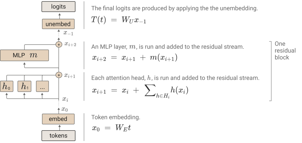
A nice way to think about these models, inspired by Elhage et al., is that we have a stream of data that is being added to by the multi-head attention and MLPs and is normalized by the layer normalizations. This stream is almost entirely linear, and it serves as an important communications channel throughout the model. The dimensions of this stream are also never changed throughout the entire model.

Multi-Head Attention

We can think of the function of multi-head attention as moving information in the residual stream and applying some weight matrices. Let’s start with a single attention head:

Scaled Dot Product Attention for One Attention Head

The transformers architecture implements scaled dot product attention. This is in contrast to additive attention, which was described in the last post. In additive attention, we have an entire alignment model (a small MLP) that computes the logits that get fed into the softmax to determine the weighting of the values. In dot product attention, we replace that alignment model with dot products and linear transformations!

If you read the original transformers paper, you will see scaled dot product attention written in the most general form as:

Let’s ignore what the \(Q\), \(K\), and \(V\) matricies represent for the moment. Initially, this notation was a bit confusing for me at first because, technically the softmax function is a vector function. The key insight is that the softmax acts on the rows of the \(Q K^\top\) matrix. Things are more clear when they are written as follows:

Essentially, we are just taking some convex combination of the rows of \(V\) in each row of our attention matrix.

Relation to Additive Attention

As a refresher, additive attention from the previous post looked like this:

Where \(\textbf{c}_i\) was the \(i\)th context vector, \(a\) was the alignment model, \(\textbf{s}_{i-1}\) was the previous hidden state of the decoder, and \(\textbf{h}_j\) was the \(j\)th output from the bidirectional RNN encoder. We can summarize the equations above as follows (note that the \(T_x = n\) from the previous post and just represents the input length):

If we take \(Q = \textbf{s}_{i-1}\) and \(K = V = H\) we can write:

In principle, all both of these attention mechanisms do is take convex combinations of the rows of some value matrix! The main difference is just how the convex combination weights are calcuated. Additive attention uses a small MLP alignment model, and dot product attention uses dot products. In fact, if \(a(\textbf{x}, Y) = \frac{\textbf{x}^\top Y^\top}{\sqrt{d_k}}\) the formula above exactly describes scaled dot product attention for one token. The transformer paper claims that while these are similar in theoretical complexity, dot-product attention is much faster and more space efficient on modern hardware. I find it incredible how we can basically just replace a small neural network with a dot product and maintain good performance 🤯.

Why Scaled Dot-Product Attention?

You might be wondering why this is called scaled dot-product attention. That is because of the \(\frac{1}{\sqrt{d_k}}\) term in the softmax. The paper claims this is because additive attention outperforms dot product attention for large values of \(d_k\) without the scaling. They suspect this is becuase the dot products grow large in magnitude, pushing the softmax function into regions of extremely small gradients, which slows gradient descent. Let’s disect why this is true, why do the dot products grow large in magnitude and why does this push the softmax function into regions of small gradients?

We can think of a dot product between two vectors of dimension \(d_k\) as \(\textbf{v} \cdot \textbf{w} = \sum_i \textbf{v}_i \textbf{w}_i\). If each entry in these vectors is a random variable with mean 0 and variance 1, then because variances add, the dot product will have mean 0 and variance \(d_k\). This is of course an oversimplification because the entires of our queries and keys will not be random variables with mean 0 and variance 1, but it illustrates the fact that as \(d_k\) grows, so does the variance of our dot product. Now how does this impact the gradient of the softmax function (technically gradients are only defined for scalar functions, so from now on I will refer to the derivative of the softmax function). Here is the derivative of the \(i\)th output with respect to the \(j\)th input.

Due to the exponent, when there is a large term in the input vector to the softmax, it ends up dominating the output probability distribution. Therefore, if we have large dot products from before, the input to the softmax is going to have some terms that are very large. In both cases for the derivative, it is likely that either \(\text{softmax}(\textbf{v})_i\) or \(\text{softmax}(\textbf{v})_j\) will be small, making the overall derivative also very small.

However, by adding the scaling term that is proportional to \(\sqrt{d_k}\), where \(d_k\) is the dimension of the dotted vectors, we make the values in the input vector to the softmax less extreme, and therefore make it less likely that the overall derivative is very small.

Multi-Head Attention

Instead of just using one attention head as in the original attention paper, the authors found it beneficial to linearly project the queries, keys, and values \(h\) times to a lower dimensional space, run attention on each, and aggregate the results.

Where \(W_i^Q \in \mathbb{R}^{d_{\text{model}} \times d_k}\), \(W_i^K \in \mathbb{R}^{d_{\text{model}} \times d_k}\), \(W_i^V \in \mathbb{R}^{d_{\text{model}} \times d_v}\), and \(W^O \in \mathbb{R}^{h d_v \times d_{\text{model}}}\). Additionally, they set \(h=8\) and \(d_k = d_v = d_{\text{model}}/h = 64\). The computational cost of this is similar to if they had just used a single head attention with full dimensionality.

Multi-Head Self-Attention in the Encoder

The way this multi-head attention plays out in the encoder is as self-attention, meaning that the queries, keys, and values all are equal to the hidden state \(H\).

One reasonable question is, why do we even need multi-head self-attention? One thing attention gets you is the ability to mix information between tokens. This is the only part of the architecture that has this capability.

Layer Normalization

Layer normalization is a commonly used method to reduce training time by normalizing hidden states within a single training example. Nowadays, it seems more commonly used than batch normalization because it is able to be used for online learning tasks or places where it is impossible to have large mini-batches, and is difficult to apply to RNNs. Here is a mathematical explanation of how it works in transformers:

First we compute the mean and variance of each of the n tokens of the our training (or test) sample:

Where \(\mu_{t}\) represents the mean for token \(t\) and \(H_{t, i}\)

The rest of layer normlization was quite suprising to me. We also add \(\gamma, \beta \in \mathbb{R}^{d_{\text{model}}}\) terms that get learned through backprop and are applied as follows:

MLP

The MLP layers of the transformer are applied identically to each token in the hidden state, and are added back into the residual stream. These layers are essentially comprised of two affine transformations with a ReLU (GeLUs are usually used in many modern models, but not in the original paper) in the middle. This can be written as follows:

One obvious question might be, what do these MLPs do? Recent work from Anthropic suggests that in language models neurons in MLPs may represent certain rules or categories such as phrases related to music or base64-encoded text. From my own work, it seems that, at least in early layers, of Vision Transformers, MLP neurons often correspond to certain visual textures or patterns.

Layer Normalization

After the MLP, there is another LayerNorm, which is applied identically to the one before.

Final Encoder Output

What was described above was one encoder block. Note that the input dimensions and output dimensions of each transformer block are the same, namely \(H \in \mathbb{R}^{n \times d_{\text{model}}}\). Therefore, we can just take the output of our first block, and feed it into our second block. This is done \(N\) times. The final hidden state that comes out of the encoder blocks then becomes the key and value matrices for the decoder \(K_E, V_E = H\), more on this later. The encoder is only ran once.

Pre Decoder

In the original transformers paper, the decoder is used autoregressively, meaning that output translations are fed back into the model. Initially, nothing except for a start of sentence token <SOS> is fed into the model. But as the model starts making predictions, the input sequence to the decoder grows. The input into the encoder is processed the same way as the input to the encoder (see the pre-encoder section).

Our current output sentence is "Bobby mag", which is tokenized as ["<SOS>", "Bobby<EOW>", "mag<EOW>"] using BPE with vocabulary size $C = 37000$. Now we can vectorize this list to get $\begin{bmatrix} \textbf{e}_{41}^\top \\ \vdots \end{bmatrix} = \begin{bmatrix} \textbf{x}_1^\top \\ \vdots \end{bmatrix} = X \in \mathbb{R}^{n \times C}$, where $\textbf{x}_i$ is the one hot vector for the $i$th input word. We again embed the words and add positional encodings as follows, $H = X U^\top + PE \in \mathbb{R}^{n \times d_{\text{model}}}$.

(Please note that the output tokens are again from BPE and your one hot vectors depend on your input and I'm just arbitrarily choosing plausible values.)

Decoder

The decoder is almost exactly the same as the encoder, except the attention works differently. Instead of just one multi-head self-attention block, we have a masked multi-head self-attention block and a multi-head attention block. So all in all, we have our embedding, then masked mutli-head self-attention, then layer norm, then multi-head attention, then layer norm, then an MLP, and finally one last layer norm.

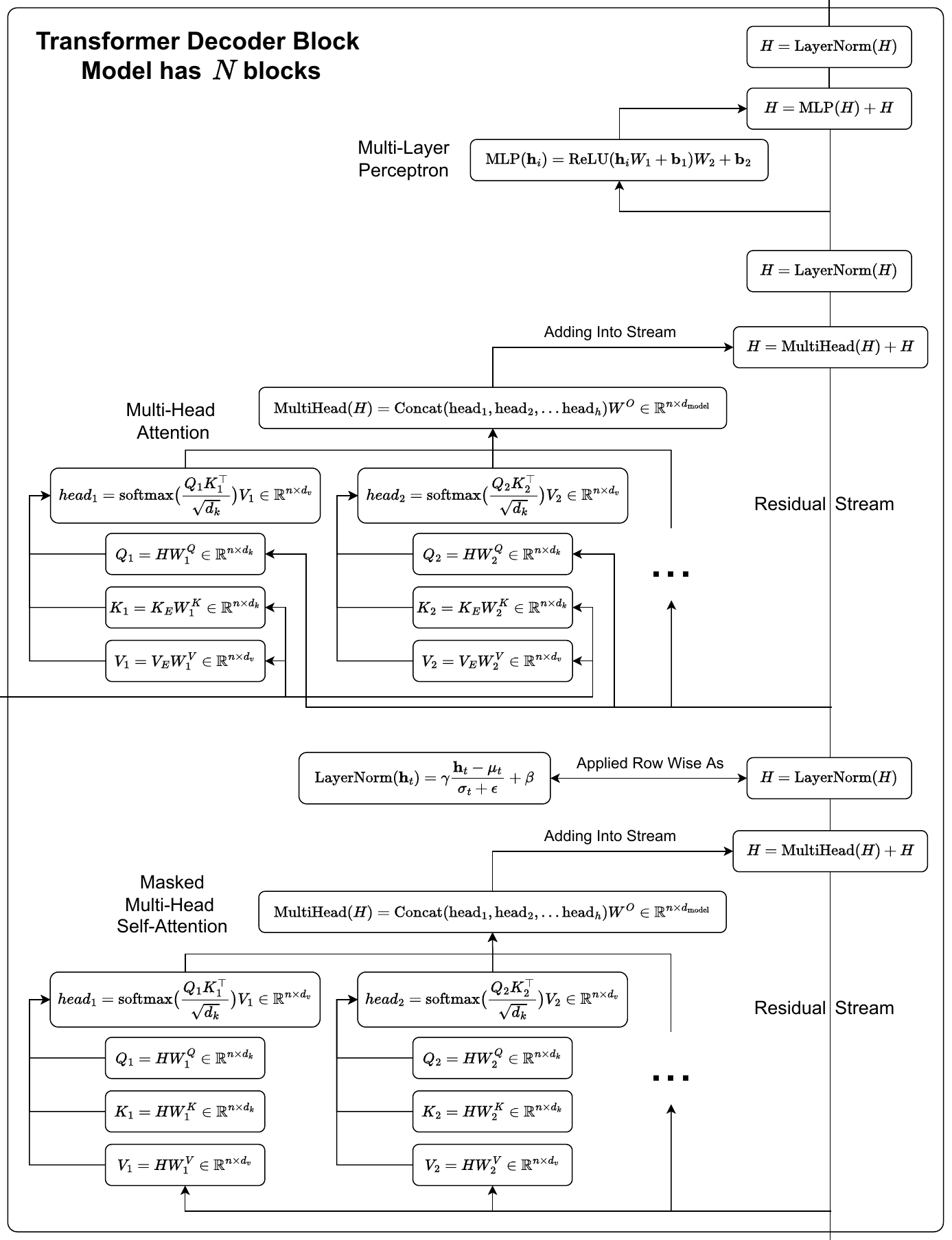Please note: There is a slight abuse of notation in the diagram above, the query, key, and value weight matrices in the masked attention and the regular attention can have different values, but are just denoted the same.

Masked Multi-Head Self-Attention

Instead of using regular multi-head self-attention, the decoder uses masked multi-head self-attention. Masked multi-head self-attention doesn’t allow for tokens to attend to later tokens. This is implemented by making out (setting to \(-\infty\)) all values in the input of the softmax which would cause attention to later tokens. This just requires us to slightly modify our equation for attention and add in a “look ahead mask”.

The paper claims masking is necessary “to prevent leftward information flow in the decoder to preserve the auto-regressive property.” To be more precise, I think the word “prevent” should be replaced with “reduce”. The reason being that technically, even for the first attention head, the tokens of the value matrix don’t have to precisely correspond to tokens. This is because the value weight matrix applies some linear transformation to the hidden state. This transformation could mix information between tokens, such that even if it is impossible for the softmax to produce connections to later tokens, the tokens representations themselves could have information from later tokens. That being said, in practice, it seems that this still enables the transformer to preserve auto-regressive property because the model works!

If we didn’t train in parallel, we actually wouldn’t need masking at all. This is because we could technically do all our training recurrently, where with each token we autoregressively generate, we save the hidden state for that token, and then use it when generating the next token (more on this later).

Multi-Head Attention

This multi-head attention block is almost the same as the multi-head self-attention in the encoder, except that the key and value matrices come from the output of the encoder. Taking the keys and values from the encoder is necessary in order to incorporate information from the the input sentence into the output translation.

Note, because the value matrix is not the current decoder hidden state \(H\), if the number of tokens in the encoder and decoder were different, we would not be able to add back into the residual stream! Therefore, in practice, a default max number of tokens, or context size, \(n\) is set (to 128 for instance) for both the encoder and decoder blocks. If the sequence is not \(n\) tokens long, the remaining tokens are filled in by padding <PAD> tokens.

Post Decoder

Just like with the encoder, there are \(N\) of decoder blocks. To get our output logits using the hidden state \(H\) passed through the transformer decoder layers, we use the embedding matrix \(U\) to unembed the hidden representation. Our logits are the \(U^\top \textbf{h}_i \in \mathbb{R}^C\). Note how we choose \(i\)th token vector to get our output logits. \(i\) corresponds to the last token in the decoder input which is not a padding token, and we get the logits from this token because we want to predict the next word after this last word. Now we can pass through a softmax to get the output probability distribution over our vocabulary. To actually get the prediction, we sample from this distribution. In the paper they play around with beam search for some of their results, but I’m just going to keep things simple and take the \(\text{argmax}\) from the distribution over our vocabulary.

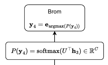
The decoder is run autoregressively until it outputs the <EOS> token, at which point the translation is finished!

We now have our final representation $H$ that has information about the original sentence in English ("Bobby likes blackberries."), the current German translation ("Bobby mag"), and the probable next word. We will first apply the unembedding to the third row of $H$ as follows, $P(\textbf{y}_4) = \text{softmax} (U^\top \textbf{h}_3) \in \mathbb{R}^C$. Now we can sample from this distribution to get $\textbf{y}_4 = \textbf{e}_{\text{argmax} (P(\textbf{y}_4))} \in \mathbb{R}^C$. If the model was trained well, this $\textbf{y}_4$ standard basis vector will likely corresponds to the token "Brom", which is the correct next token in the translation.

Training a Transformer

To train the described configuration of the transformer, the authors used the WMT 2014 English-German dataset. The Adam optimizer was also used with \(\beta_1 = 0.9, \ \beta_2 = 0.98, \ \epsilon = 10^{-9}\). Additionally, they increased the learning rate linearly for the first 4,000 training steps, and then employed inverse square root learning rate decay for the remaining 96,000 training steps. Here is the mathematical formula used: \(lrate = d_{model}^{-0.5} \cdot \min ( step\_num^{-0.5}, step\_num \cdot warmup\_steps^{-1.5} )\)

If you are curious about the details of why learning rate decay works, please see this great paper.

They also used residual dropout, applied to the output of each sub-layer and the input into the encoder and decoder (the sums of the embeddings and positional encodings).

The paper has details on the performance.

Variants on the Original Architecture

There are several variants on the original transformer architecture, most notably encoder only transformers (like BERT) and decoder only transformers (like GPT).

Encoder Only Transformers

There is a class of transformer models that are often referred to as encoder only transformers. Most commonly, this refers to BERT models. BERT stands for Bidirectional Encoder Representations from Transformers. BERT essentially just takes the encoder part of the transformer, scales it up and fine tunes it on downstream tasks. The encoder is bidirectional because it lacks any sort of masked attention. This enables the model to use information from further down in the sentence to create representations for an earlier word.

One of the main tasks this model is pretrained on is masked language modeling, where the model is fed an input sentence with a random word masked out, and the model has to figure out what the word is. Here is an example input sentence and the appropriate output.

Input: “Tommy, who loves soccer, just <MASK> a goal.” Desired Output: “Tommy, who loves soccer, just scored a goal.”

However, in 2023, the hype is much more around decoder only transformers.

Decoder Only Transformers

Decoder only transformers take the original transformer architecture, throw away the encoder, and only keep the decoder. The multi-head attention is removed and we only keep the masked multi-head self-attention because we no longer can get the key and value matrices from the encoder. This architecture can be trained with next token prediction, where the model is fed part of a sentence, and tries to generate the next word. At test time, the model autoregressively generates the output sentence.

A series of popular decoder only transformers is the GPT series of models (GPT, GPT-2, GPT-3, and soon GPT-4). With the original GPT, the paradigm was still to pretrain the model on lots of general data, and then fine tune it for specific tasks. Nowadays, the paradigm has gone away from fine tuning and to prompting. There are many resources online which explain this and you can play around with it yourself with Chat-GPT.

Conclusion

I hope this post sheds a bit of light on how transformers work! There are still many questions I haven’t answered here (some of which have answers in the literature, some of which don’t), such as: Why are transformers better than other architectures? How can transformers be used with other modalities? What algorithms do transformers learn? What are the limitations of the transformer architecture? How far will scaling take us?

I might try to answer some of these in a future blog post. But for now, stay calm and code on 😎.

References:

• Attention Is All You Need
• Last Post on Attention
• A Good Implementation
• Transduction in ML
• Understanding LSTMs
• Byte-Pair Encoding Paper
• Byte-Pair Encoding explanation
• Using the Output Embedding to Improve Language Models
• Illustrated Transformer
• A Mathematical Framework for Transformer Circuits
• Vanishing Gradients Problem
• Derivative of Softmax
• What are the queries, keys, and values?
• Layer normalization
• Papers With Code Layer Norm
• Batch Normalization
• Mathematical Explanation
• GeLUs
• SoLU
• Understanding Masked Multi-Head Attention
• How Does Learning Rate Decay Help Modern Neural Networks?
• BERT models
• Decoder only transformers
• GPT
• GPT-2
• GPT-3
• GPT-4 Announcement
• Chat-GPT
• The Annotated Transformer
• A Mathematical Guide to Transfomers