WARNING: This post assumes you have a basic understanding of neural networks and specifically Convolutional Neural Networks (CNNs). Some Python knowledge (PyTorch and NumPy mainly) would also be useful to understand the code samples.

This post is the written extension of a presentation given for a deep learning theory reading group at Columbia.

This post is an explanation of some of the basics of Grad-CAM. There are, however, some things described in the paper that are not mentioned here. I will start by giving an overview of CNN interpretability and describing the basics of Grad-CAM. Then I will explain how CAM works. Finally, I will get back to Grad-CAM and give a more detailed explanation.

My implementation in PyTorch on the MNIST dataset is in a jupyter notebook and can be found in html form here. The GitHub repo can be found here. I will show some of the result images and code here.

Very Basics of Interpretability

Simply put, interpretability matters. And it matters for a variety of reasons. You could look at it from the perspective of AI Safety, if we have more intepretable models, perhaps we can find unknown safety problems in our models that can prevent doom. This is something I may explore more in a future blog post :)

For now though, I’m going to explain the more near term reasoning the authors of the Grad-CAM paper said for why interpretability matters. Namely they said that in order to build trust in AI systems for more meaningful integration into our lives, we need more transparent models. They mentioned how this can be useful at 3 stages of AI development in a problem:

1. When AI is much weaker than humans at a task, intepretability helps to identify failure modes that can help to find directions to improve the model.
2. When AI is on par with human performance on a task, interpretability can help build trust.
3. When AI is better than humans at a task, interpretability can help enable machine teaching where humans can learn from AI systems.

One thing Grad-CAM tries to address, is the traditional accuracy and simplicity/interpretability trade-off. Basically, if you think of models that were more popular in the past such as decision trees, they were very interpretable, but not very accurate at many tasks such as image classification or sentence translation. However, if you look at more modern deep neural networks, they can have incredible accuracy, but are often complex black boxes that are very hard to interpret. Grad-CAM aims to be an interpretability tool that can beat this trade-off.

Another thing that Grad-CAM tries to do is to be a good visual explanation. The authors claim that a good visual explanation is high resolution and class discriminative. We will explore how Grad-CAM is both of these.

Now we are ready to dig in. However, before talking about Grad-CAM we will discuss CAM.

Class Activation Mappings (CAM)

CAM aims to create class-discriminative localization maps that essentially show what the CNN looks at when making a certain classification. These heatmaps look like this:

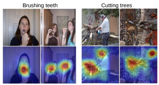
In the class activation mappings, the authors cited two key recent discoveries at the time (this paper was written in late 2015) that helped their research.

The first is that Zhou et al showed that various layers of convolutional neural networks actually behave as object detectors. The key word in that sentence is detectors, because the detection problem involves classification and localization. So essentially there is localization ability built into these convolutional layers, but it turns out that this ability is lost when fully-connected layers are used after the convolutional layers.

The second discovery is that some popular fully-convolutional neural networks came out at the time that totally avoided using full-connected layers to minimize the number of parameters, and instead use global average pooling. This global average pooling acts as a regularizer and has also been shown to retain the localization ability described before until the output layer.

However, before describing the rest of CAM, I first want to explain Global Average Pooling (GAP).

Global Average Pooling

When GAP is used, it is typically applied to the output of the final convolutional layer. It collapses the \(h \times w \times d\) output down to a \(1 \times 1 \times d\) vector. One slightly weird thing is that in the CAM paper they don’t actually take the average of each of the \(d\) feature maps that come from the final convolutional layer, they just take the sum of all. Notation alert: I’m going to use notation that is more consistent with the Grad-CAM paper.

\(F^k = \sum_{i} \sum_{j} A_{ij}^k\)

• Where \(k \in \{ 1, 2 \ldots d \}\) representing the \(k\)th feature map from the final conv layer
• \(F^k\) is just a number and represents GAP applied to the \(k\)th filter

This picture shows what’s going on:

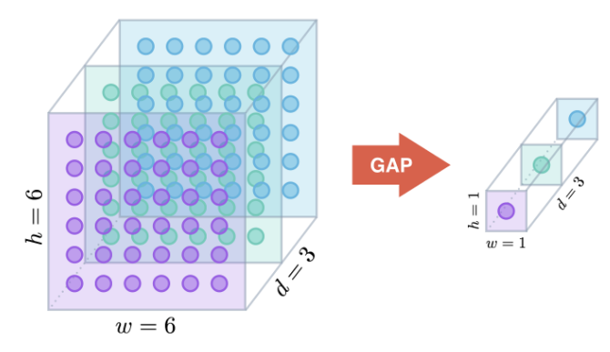
I implemented this as follows in PyTorch into my model for classifying MNIST digits.

class CAM_CNN(nn.Module):
  def __init__(self):
    super(CAM_CNN, self).__init__()

    self.conv1 = nn.Sequential(         
      nn.Conv2d(
        in_channels=1,              
        out_channels=16,            
        kernel_size=5,              
        stride=1,                   
        padding=2               
      ),                              
      nn.ReLU(),                      
      nn.MaxPool2d(kernel_size=2)   
    )

    self.conv2 = nn.Sequential(         
      nn.Conv2d(16, 32, 5, 1, 2),
      nn.ReLU(),
      nn.MaxPool2d(2)
    )

    self.gap = nn.AvgPool2d(7) # GAP here!

    self.out = nn.Linear(32, 10)


  def forward(self, x):
    x = self.conv1(x)
    x = self.conv2(x)
    y = self.gap(x)

    y = y.view(y.size(0), -1)

    y = self.out(y)
    return y, x

Back to CAM

Now we can come back to CAM. CAM requires a sort of specific architecture to work. It requires the network consists of convolutional layers (these can have any sort of pooling, dropout, residual blocks etc.), then a GAP layer, and finally an output layer.

CAM relies on the fact that we can identify the importance of certain regions of the image by projecting the weights of the output layer back onto the final convolutional feature maps. Essentially to get the CAM, we take a weighted average of the final convolutional feature maps weighted by the weights of the output class that connect to the global average pooling.

\(L_{CAM}^c=\sum_k w_k^c A^k\)

• Where \(L_{CAM}^c\) represents the CAM of output class c.
• \(w_k^c\) represents the \(k\)th weight of output class \(c\).

Maybe this picture from the paper can help make things more clear:

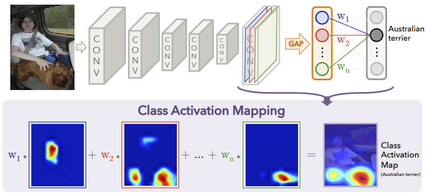
Because typically as you go though more and more convolutional layers the width and height of your feature maps decrease and your depth increases, you will likely have to upscale the CAM to the size of your image so you can nicely overlay it.

In PyTorch I implemented this as follows, where sum_res is the final class specific CAM representation and has dimensions of [10, 7, 7].

with torch.no_grad():
  x, y = data[data_index][0], data[data_index][1]
  
  final_conv_output = 0
  cam_weights = 0

  pred, final_conv_output = model(x[None, :])

  for param in model.parameters():
    if param.size() == torch.Size([10, 32]):
      cam_weights = param
      break

  mult_res = torch.mul(cam_weights[:, :, None, None], final_conv_output)

  sum_res = torch.sum(mult_res, 1)

GAP vs GMP

A question that might come up is, why GAP and why not Global Max Pooling (GMP). In the paper, they cite emiprical evidence that says that GAP and GMP have similar classification performance, but GAP has better localization performance. Also intuitive reasoning says that GAP will encourage the network to identify the extent of an object while GMP encourages it to find one disciminative feature.

Uses

CAM is already pretty useful! It can lend insights into failure modes (such as this famous US Army story that may or may not be true). Another thing is that it can be used as a weakly supervised model (as opposed to a strongly supervised model given bounding boxes during training time) for object localiation. The idea is that you basically draw bounding boxes around the CAM visualizations per class to get your localization. It actually performed decently well (see paper for more details).

From my personal implementation, I understood how CAM can do both of these things. One detection that my model got wrong is this 6:

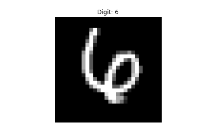
At first glance to me, it seems kind of obvious that it’s a 6. However, when I looked at the CAM visualization it became more clear how the model could mistake it for a 4.

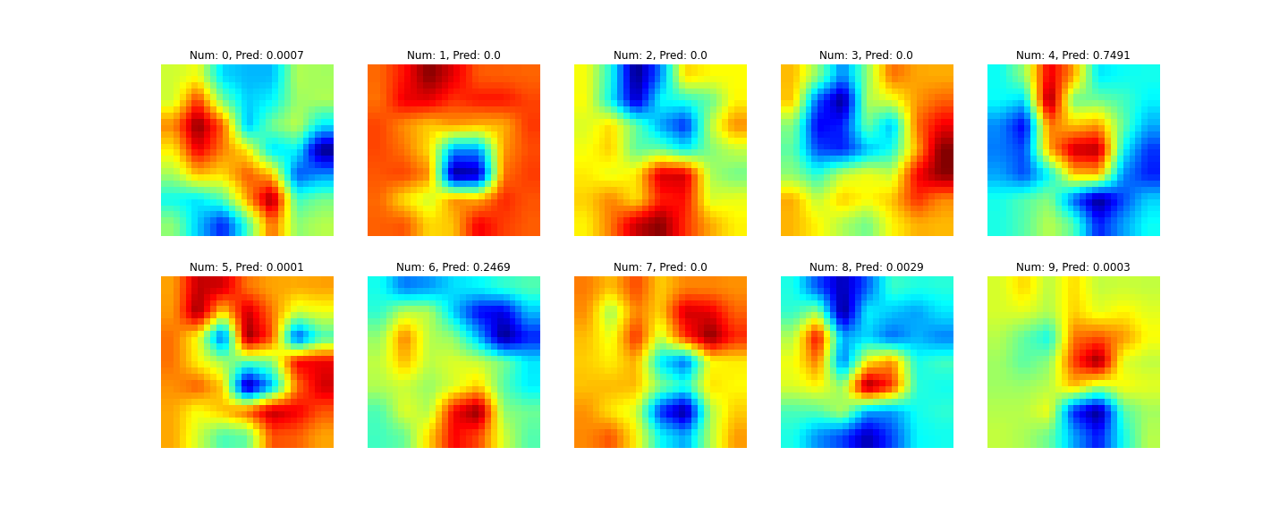
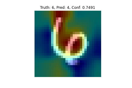
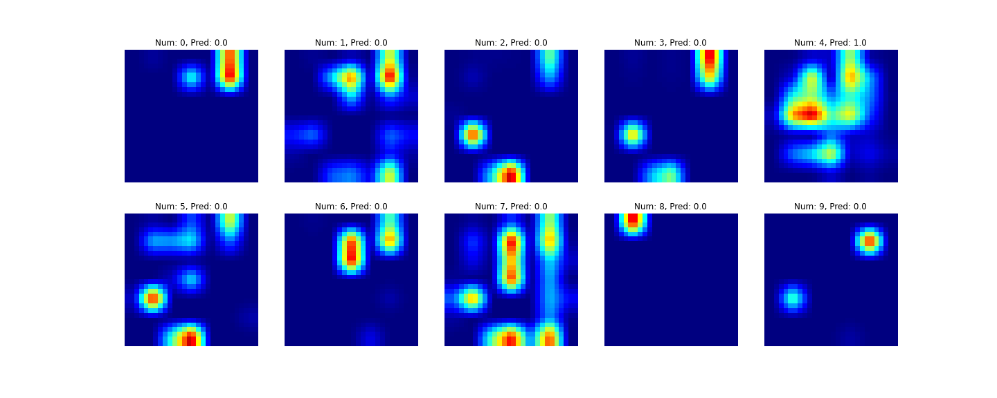
The top images shows the CAM heatmaps for all classes and the bottom image shows the predicted class overlaid onto the input image. For classes that don’t have a high output probability, the visualizations are less interesting, but for ones that are higher such as 6 and 4 in this example, it is more interesting. The redder regions represent regions that positively correlate with that output class. So you can see how for detecting a 4, the model doesn’t look that much at the bottom part of the 4. This can be confirmed by looking at correct detections of 4’s where the same trend can be spotted.

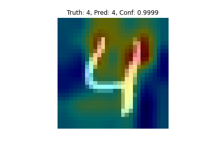
Now looking back at the original 6, it is more understandable how the model could mistake it for a 4, if it’s definition of a 4 doesn’t value the bottom part of the 4 much.

CAM also seemed to work pretty well as a weekly supervised object localization model. Of course, in the MNIST dataset, location doesn’t matter too much as the digits are mostly centered, but it’s still clear by this example of a 7 that the model seems to do a good job of this:

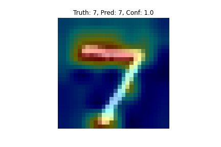
If you drew a good bounding box around the redder regions of the image, you would localize the 7 pretty well. Another cool thing you can see here is that the model doesn’t seem to value what happens around the middle of the slanted line in the 7, this could be because some of the 7’s in the dataset contain dashes there and some don’t, so the model might have learned not to really pay attention to that.

Areas of Improvement

However, CAM is by no means perfect. For one, the output visualizations are not very high resolution due to the upscaling step. Additionally, CAM only works for a relatively small set of possible models, which means it is still stuck in the accuracy vs interpretability trade-off as there could be other models with better accuracy that CAM can’t be applied on, meaning they are less interpretable. Further issues that both CAM and Grad-CAM have will be discussed below.

Gradient Based Class Activation Mappings (Grad-CAM)

Now we can finally talk about Grad-CAM! The basic idea is the same as CAM, we are again trying to obtain class-discriminative localization maps. Only now, we are using gradient information (hence Gradient Based CAM) flowling into the last convolutional layer to get importance values for each neuron for a particular decision. This is instead of using the weights to the output layer from GAP as seen in CAM. Due to the nature of gradients, Grad-CAM can be used for any convolutional layer. However, it is typically uses the last convolutional layer because deeper representations in CNNs have been found to capture higher level visual concepts which is what we are after.

Simply put, this is what Grad-CAM does:

\(L_{Grad-CAM}^c=ReLU(\sum_k \alpha_k^c A^k)\)

• We apply the ReLU because we only care about features that have a positive influence on the class of interest, negative features likely belong to other classes.
• Basically substituting \(w\) for the \(\alpha\) term.
• \(A^k\) is the \(k\)th feature map of the final convolutional layer outputs.

The \(\alpha_k^c\) term comes from here:

\(\alpha_k^c = \frac{1}{Z}\sum_i \sum_j \frac{\partial y^c}{\partial A_{ij}^k }\)

• \(y^c\) represents the output of the final layer before the softmax for a specific class.
• \(Z\) is a proportionality constant used for normalization (it is the number of pixels in the feature map).
• \(\alpha_k^c\) represents a partial linearization of the deep network downstream from \(A\).

You can see how this \(\alpha\) term is very similar to GAP. We are taking the average of the gradients of the output class with respect to each pixel in the \(k\)th feature map, essentially giving us the “importance” of that feature map to the final prediction.

The paper further shows how Grad-CAM is actually a strict generalization of CAM.

In my personal implementation, I used the following model (note how it doesn’t have the GAP like my CAM implementation model had).

class Grad_CAM_CNN(nn.Module):
  def __init__(self):
    super(Grad_CAM_CNN, self).__init__()

    self.conv1 = nn.Sequential(         
      nn.Conv2d(
        in_channels=1,
        out_channels=16,
        kernel_size=5,
        stride=1,
        padding=2,
      ),
      nn.ReLU(),
      nn.MaxPool2d(kernel_size=2),
    )

    self.conv2 = nn.Sequential(
      nn.Conv2d(16, 32, 5, 1, 2),
      nn.ReLU(),
      nn.MaxPool2d(2),
    )

    # fully connected layer, output 10 classes
    self.out = nn.Linear(32 * 7 * 7, 10)

    self.input_gradients = None

  def input_gradients_hook(self, grad):
    self.input_gradients = grad
  
  def get_input_gradients(self):
    return self.input_gradients

  def forward(self, x):
    x.requires_grad_()
    x.retain_grad()

    x.register_hook(self.input_gradients_hook)

    x = self.conv1(x)
    x = self.conv2(x)
    
    # flatten the output of conv2 to (batch_size, 32 * 7 * 7)
    y = x.view(x.size(0), -1)
    y = self.out(y)
    
    return nn.functional.log_softmax(y, dim=1), x

To get the actual Grad-CAM visualizations, I did the following:

model.eval()

x, y = data[data_index][0], data[data_index][1]

class_specific_alphas = torch.tensor((), dtype=torch.float64)
class_specific_alphas = class_specific_alphas.new_zeros((10, 32))

for c in range(10):
  model.zero_grad()
  pred, final_conv_output = model(x[None, :])

  final_conv_output.requires_grad_()
  final_conv_output.retain_grad()

  one_hot_output = torch.FloatTensor(1, pred[0].size()[-1]).zero_()
  one_hot_output[0][c] = 1

  pred.backward(gradient=one_hot_output, retain_graph=True)

  class_specific_alphas[c] = torch.sum(final_conv_output.grad.squeeze(), (1, 2))

class_specific_alphas = torch.div(class_specific_alphas, 7 * 7)

pred, final_conv_output = model(x[None, :])

mult_res = torch.mul(class_specific_alphas[:, :, None, None], final_conv_output)
sum_res = nn.functional.relu(torch.sum(mult_res, 1))

Where sum_res is once again the final class specific CAM representation and has dimensions of [10, 7, 7].

Now here you might be thinking, why is this guy using \(y^c\) after the softmax, I thought it was supposed to be before the softmax? And you would be right, the paper does say before. However, I found that using $y^c$ after the softmax worked better. I believe this is because when calculating the gradient backwards I am setting the output to 0 for all classes and 1 for the target class. However, without the softmax, the outputs of the model are very far away from 0 and 1 for the other and target classes. I think (I am not sure) that this results in the final Grad-CAM output having most values that are 0 or less as the typical output for the target class is much higher than 1 and for the other classes is much less than 0 so the gradients are negative. Then when applying the ReLU to the Grad-CAM some images were just totally 0. But with the softmax applied the final outputs look much better. Perhaps some sort of normalization within the network could help.

Guided Grad-CAM

So far, Grad-CAM seems great! Because of the gradients we can now apply this visualization technique to a much wider range of models, sort of allowing us to beat the accuracy vs interpretability trade-off. But another thing we wanted to achive is to obtain high resolution visual explanations. To do this, we need Guided Grad-CAM.

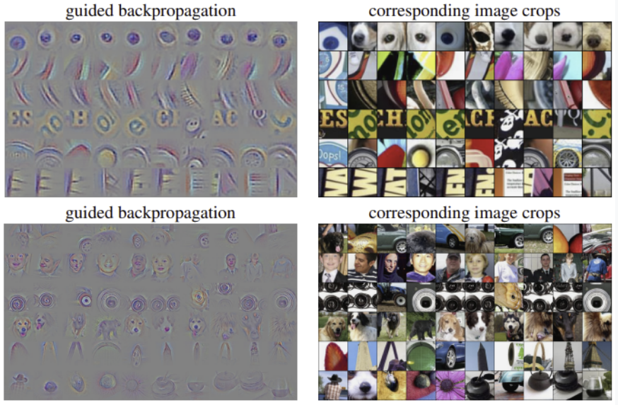
Guided Grad-CAM relies on Guided Backpropagation. Guided backprop is actually a very simple concept. We are trying to find how each pixel in the input for a specific class contributes to the output. Therefore we can propagate the gradient backwards all the way back to the input image. However, we want to set all negative gradients to 0 because we only care about pixels that positively influence our outputs. This gets us an image which for each pixel essentially represents how much that pixel influences the output. It looks like this:

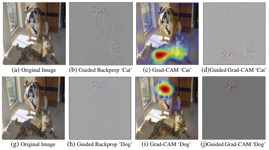
The thing about guided backprop is that it is not class discriminative. We can, however, take the outputs from guided backprop (which is high resolution) and elementwise multiply it by the upscaled class discriminative Grad-CAM visualizations to get Guided Grad-CAM which is both high resolution and class discriminative! This is what that looks like:

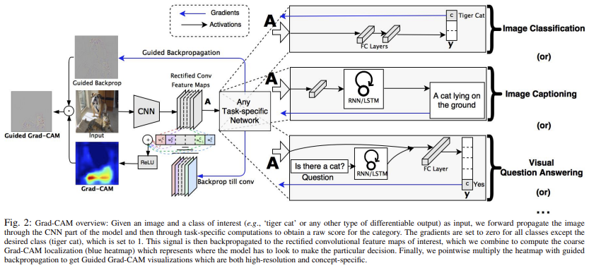
The Grad-CAM paper describes many other things including Grad-CAM for visual question answering, weakly-supervised localization and segmentation, and more. I won’t go into these but I will show one cool picture that gives a good overview of Grad-CAM.

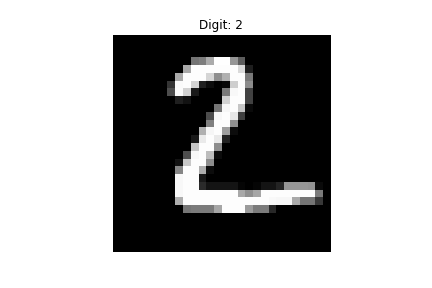
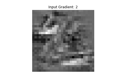
In my implementation, I’m not actually implementing guided backprop. I am just computing the gradients of the inputs w.r.t. the output predictions, I am not applying a ReLU to the gradients as they are propagating backwards which is what guided backprop does. I found that for this simple MNIST example it is sufficient not to use strict guided backprop. It looks as follows:

Uses

Grad-CAM can be used for many things, I’ll just mention a few of them:

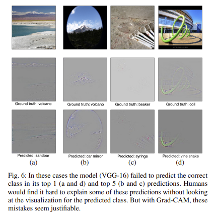
• Grad-CAM can lend insights into failure modes. This picture hows how the authors did this for the VGG-16 model.

• It can do impressive weakly-supervised object localization
• It can help identify biases in models and allow the models to achieve better generalization.

In my personal implementation, like for CAM, I found Grad-CAM useful for lending insights into failure modes and for weakly-supervised object localization. It’s impossible harder to identify the types of racial or similar biases in the MNIST dataset so I didn’t try to do that.

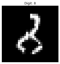
The best example for understanding a failure mode I could find was this digit which is apparently supposed to be an 8. The model detected it as a 2, however.

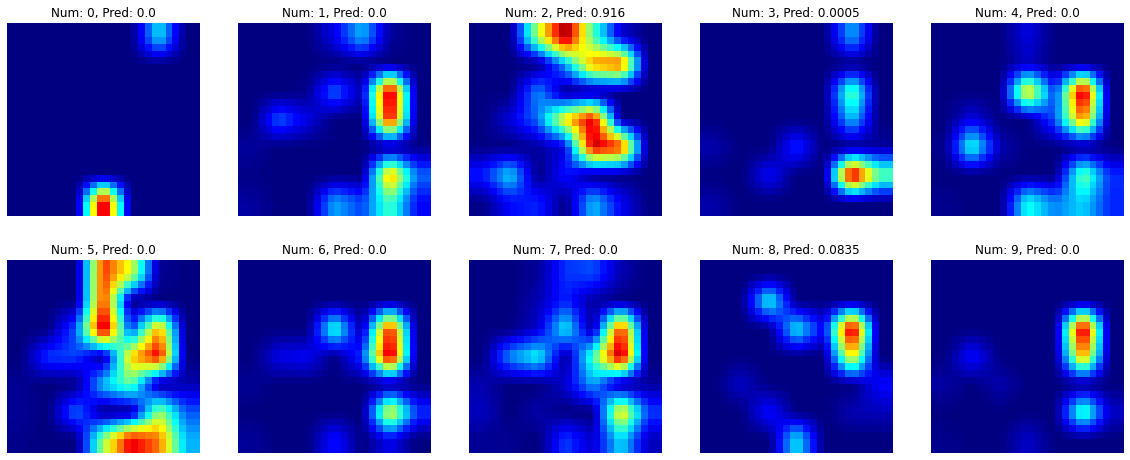
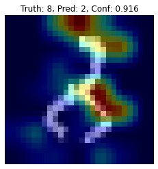
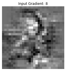
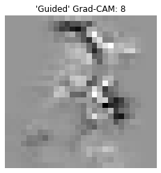
Looking at the “Guided” (I’m using quotes because it is technically not guided backprop just the gradient of the input, explained more above) Grad-CAM output, it is clear how that can be mistaken as a 2. The heatmap also shows that the model isn’t paying attention to the bottom of the digit much to classify it as a 2.

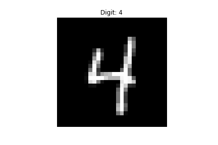
For the weakly supervised object localization it is clear that you could draw a relatively suitable bounding box to localize the character. This worked better for some input images than other in my implementation. This 4 is an example of a digit for which it worked pretty well.

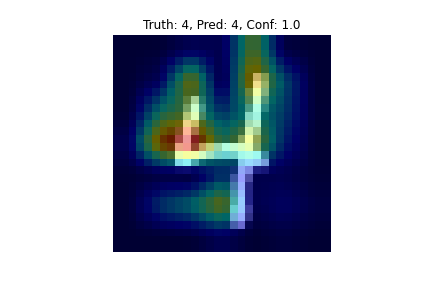
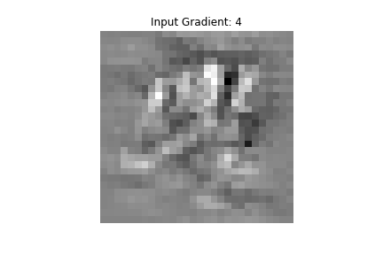
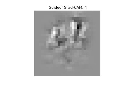
One cool thing to note is how the Grad-CAM model had better accuracy on the test data than the CAM model. This is likely due to the greater freedom for model choice that Grad-CAM allows. Of course, this is not very rigorous and I could have made my CAM model much better than my simple Grad-CAM model probably by maybe adding more conv layers or trying some regularization techniques or something, but the point is that even from this simple toy example, we can see that Grad-CAM does a better job of beating the accuracy vs. interpretability trade-off.

Areas of Improvement

Even though Grad-CAM fixes some issues that CAM had, it is still not perfect. Heatmaps are a step in the right direction, but still may fail to explain complex relationships in images. There are more modern techniques that can do a better job of this. Also Grad-CAM is only for computer vision, there are many other areas of AI that also need interpretation.

Conclusion

To me, the simplicity of Grad-CAM is really exciting. I find interpretability as a whole a really fascinating and seemingly important field and I can’t wait to read and write more about it in the future 🤓.

References:

• CAM
• Grad-CAM
• Guided Backpropagation
• Some other papers and articles were cited in the text above.

My Implementation HTML and GitHub Repo.