WARNING: This post assumes you have a basic understanding of neural networks and specifically Recurrent Neural Networks (RNNs).

There are some things in my life, that I’ve heard about many times, but never really understood. Transformers are one of those things. That’s why, in this series of posts, I’m going to give all the building blocks that took me from a decent understanding of neural networks and RNNs but no understanding of Transformers, to a basic technical understanding of Transformers. I’m going to start with the building blocks of Transformers, namely attention mechanisms. I’m going to base most of this post on the paper Neural Machine Translation by Jointly Learning to Align and Translate, which first introduced attention mechanisms in 2014 (the year Germany won the world cup 😃⚽️).

I have not yet implemented this paper, but I found this good PyTorch implementation online. I might come back to this post and add my own implementation 🙃.

I want to start by giving relevant background to the problem this paper aims to address.

Neural Machine Translation

Neural machine translation aims to take an input sentence comprised of the input words \(\mathbf{x} = (x_1, \ldots, x_{T_x})\) and translate it into an output sentence \(\mathbf{y} = (y_1, \ldots, y_{T_y})\) in a different language, where using only a single (They say single in the paper but technically their model comprises of multiple neural networks as you will soon see. I guess sometimes these things are just a little vague, but I think you get the idea), pretty large, neural network. I’m now going to introduce a recurring translation example used in the paper.

English Input Sentence:

An admitting privilege is the right of a doctor to admit a patient to a hospital or a medical centre to carry out a diagnosis or a procedure, based on his status as a health care worker at a hospital.

A Reference Translation:

Le privilege d’admission est le droit d’un medecin, en vertu de son statut de membre soignant d’un hopital, d’admettre un patient dans un hopital ou un centre medical afin d’y delivrer un ´diagnostic ou un traitement.

Warning: The accents on top of some of the letters have disappeared during the copy/paste.

Now I don’t know French. So I’m just going to trust some of the authors analysis on the accuracy of their model’s translations. However, if I were trying to implement this myself on a lot of data, it would be really useful to automatically gauge how good a generated translation is. Luckily, there is something for this, called the BLEU Score!

BLEU Score

The paper does a really good job of explaining how they derived the BLEU score, I’m just going to give a brief overview.

The core assumption that the BLEU (BiLingual Evaluation Understudy) score paper makes, is that the closer a machine translation is to a professional human translation, the better it is. So really all the BLEU score does is measure the closeness of a machine translation to one or more reference human translations.

Essentially, BLEU tries to compare \(n \text{-} gram\) (basically just sequences of \(n\) characters) in the machine translation to the reference translations. There is also an added brevity penalty to avoid translations that are just really short. The equations below are for scoring texts with multiple sentences.

Where:

• \(c\) represents the length of the candidate translation.
• \(r\) represents the effective corpus length, and is calculated by summing the best match lengths (best match length is just the closest reference sentence length, so if the candidate translation for a sentence has 12 words and there are references with 10 and 13 words, the best match length would be 13) for each candidate sentence in the corpus.

• \(N\) is usually around 4

• \(C\) represents a sentence in \(Candidates\), which contains all the sentences in the translation. Now there is a technicality here, when I say \(C\) is “a sentence”, what I really mean is \(C\) is the translation of a sentence and could technically be multiple sentences.

• \(Max \_ Ref \_ Count\) is the maximum number of times an \(n \text{-} gram\) is seen in a single reference translation.
• \(Count\) is just the number of times an \(n \text{-} gram\) is seen in the candidate translation.

I just want to take a second to sum this all up a little more intuitively. Basically, we are going over different values of \(n\) from 1 to about 4, and (in the case where we are using our simple, uniform, definition for \(w_n\)) taking the average of the number of those \(n \text{-} grams\) seen in the candidate translation and the reference translations, over the number of those \(n \text{-} grams\) in the candidate translation. Finally, we have this brevity penalty that penalizes translations that are very short. Overal this outputs a number from 0 to 1, and the higher the number is the more it is like the reference translations. This is a bit of an over simplification, but it gets the idea across.

Now that we have some background on neural machine translation and the BLEU score, we are ready to tackle attention! We will start by understanding previous approaches to neural machine translation, and then see how the attention mechanism makes it better.

Previous Approach

The previous approach mentioned in the paper is called RNN Encoder-Decoder, and was proposed by Cho et al. and Sutskever et al..

Encoder

Essentially, this model works by first having an encoder that reads in the input sentence \(\mathbf{x}\) and outputs a fixed-length vector \(c\) called the context vector (more on this later). This can be done as follows:

The paper describes how the previous approaches used an LSTM as \(f\) and \(h_{T_x} = q(\{h_1, \ldots , h_{T_x} \})\). Hopefully, you can see how this makes sense given your background RNN understanding. It’s pretty much a many to one RNN, where we are just reading in the sentence word by word and outputting the hidden state after the final word is read in to the decoder.

Decoder

The decoder aims to predict the next word \(y_{t'}\) given the context vector \(c\) and the previously predicted words \(\{y_1, \ldots, y_{t'-1} \}\). The decoder basically defines a probability over a translation \(\mathbf{y}\) that goes as follows, decomposing the joint probability into ordered conditional probabilities:

RNNs allow us to model each conditional probability as:

where \(g\) is an RNN (GRU, LSTM, whatever) and \(s_t\) represents the hidden state. This is just a one to many RNN that takes an input context vector \(c\) and outputs a translation \(\mathbf{y}\).

Issues

The biggest problem that the authors mention with this model is the fact that it uses a fixed length context vector \(c\). This forces the model to squash all the information from the input sentence, into a set length vector. The problem is this sentence can be of different lengths. The attention mechanism that is proposed in this paper frees the mode from this fixed length context vector \(c\) and is shown to achieve much better performance on longer sentences.

New Model

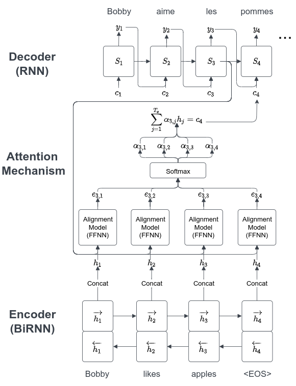
The new mechanism that they claim learns to align and translate uses the attention mechanism and looks as follows:

Decoder

Instead of defining each conditional probability as in Eq. 9, we can define them as follows:

\(g\) is just some RNN model again. To output a word \(y_i\), you just need to sample from the conditional distribution.

\(s_i\) is just the hidden state at time \(i\), and \(f\) is another part of whatever RNN architecture is being used.

Note how the \(c\) term (context vector) now has a subscript! This is because the context vector \(c_i\) term now depends on a sequence of annotations \((h_1, \ldots, h_{T_x})\) which the encoder creates. \(c_i\) is a weighted sum of these annotations.

Where \(\sigma\) is just the softmax function, and:

\(a\) is an alignment model which scores how well inputs around position j in the candidate sentence and the output translation at i match. Here \(a\) is just a feedforward neural network that is trained jointly with everything else.

While this may all look scary at first, all that’s really going on is that we are using \(c_i\) for the \(i\)th output word instead of \(c\). And we are calculating \(c_i\) as a weighted sum of these annotations \(h\) that the encoder creates. \(h_j\) contains information about the whole input sentence with a focus on the parts surrounding the \(j\)th word.

Pay attention to the attention mechanism here 😉!! These weights \(\alpha_{ij}\) tell the model what parts of the sentence to pay attention to when predicting the \(i\)th word. The alignment model figures out what parts of the sentence to pay attention to based on the previous hidden state \(s_{i-1}\).

The cool thing is this is kind of similar to what we people do as well. If I had to translate a short sentence from English to German (I don’t know French but I do know German), I could just read the entire sentence (encoder), store it in my brain (context vector \(c\)), and then say it in German (decoder). But if I had to translate a longer sentence, I would first try to translate the beginning of the English sentence, and pay attention to the words over there. I wouldn’t care about the words at the end of the sentence to translate the ones at the beginning.

Encoder

The encoder is responsible for creating these annotations \((h_1, \ldots, h_{T_x})\) and does so using a bidirectional RNN (BiRNN). The reason a regular RNN is not used is because a regular RNN only has information about the previous words, which wouldn’t allow annotations to have context that comes later in the sentence that could be important to the meaning of the current part of the sentence.

The BiRNN consists of a forward and backward RNNs that read the sentences in regular and reverse order respectively and calculate the hidden states \((\overrightarrow{h_1}, \ldots, \overrightarrow{h_{T_x}})\) and \((\overleftarrow{h_1}, \ldots, \overleftarrow{h_{T_x}})\) respectively. The arrows are just used to represent the forward and backward RNN hidden states. These are concatenated such that the hidden state \(h_j\) corresponding to word \(x_j\) is \(\left [ \overrightarrow{h_j^T} ; \overleftarrow{h_j^T} \right ]\). This way \(h_j\) contains context from before and after in the sentence, mainly focused near the \(j\)th word because of RNNs tendency to represent recent inputs better.

Performance

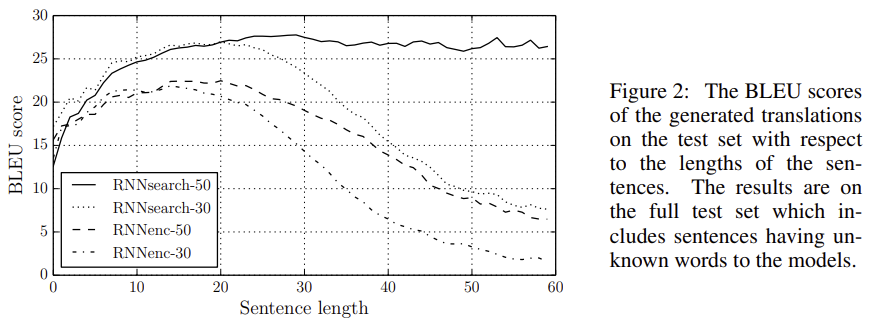
The authors of the paper trained 4 different models: RNNencdec30, RNNencdec50, RNNsearch30, and RNNsearch50, where RNNencdec is the previous model and RNNsearch is the new attention based model, and the number at the end represents the longest sentence size seen in the training data. The graph below shows the BLEU scores for these different models on different test sentence lengths. Please note how the BLEU score is greater than 1 here, it was just multiplied by 100.

The impressive thing here is that the performance for the attention based model has better performance across all sentence lengths. It is intuitively to be expected that it performs better for longer sentences given that the model avoids the fixed-length context vector \(c\), but the fact that it performs better across the board is really impressive.

Going back to our previous example from the start of the post we can see how RNNencdec-50 fails at longer sentences:

English Input Sentence:

An admitting privilege is the right of a doctor to admit a patient to a hospital or a medical centre to carry out a diagnosis or a procedure, based on his status as a health care worker at a hospital.

RNNencdec-50:

Un privilege d’admission est le droit d’un medecin de reconnaitre un patient a l’hopital ou un centre medical d’un diagnostic ou de prendre un diagnostic en fonction de son etat de sante.

RNNencdec-50 Translated Back Using Google Translate:

An admitting privilege is the right of a physician to recognize a patient at hospital or medical center for a diagnosis or to take a diagnosis by depending on his state of health.

This translation is clearly not right at the end. But the RNNsearch-50 translation on the other hand…

RNNsearch-50:

Un privilege d’admission est le droit d’un medecin d’admettre un patient a un hopital ou un centre medical pour effectuer un diagnostic ou une procedure, selon son statut de travailleur des soins de sante a l’hopital.

RNNsearch-50 Translated Back Using Google Translate:

An admitting privilege is the right of a physician to admit a patient to an hospital or medical center to perform a diagnosis or procedure, depending on his status as a health care worker at the hospital.

Impressive huh?

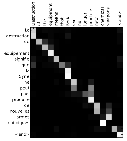
The paper also shows these plots showing the \(\alpha_{ij}\) of the \(j\)th source word for the \(i\)th target word. You can see how the model learned to pay attention to things that are intuitive for people as well. “Destruction” and “La destruction” go together but “Syria” for example isn’t important for that translation.

Conclusion

Attention is really cool and has revolutionalized much of AI. This post has reviewed the paper that first introduced attention, and introduced what is today known as additive attention. The clever way the alignment model is tied into the RNNs and to avoid the problems with fixed length context vectors and improve performance for longer input sentences is really impressive. Also the way attention is at least somewhat more biologically plausible than creating fixed length context vectors is exciting. The next post is a look at the technical details of Transformers.

References:

• Neural Machine Translation by Jointly Learning to Align and Translate
• BLEU Score
• Someone Else’s Implementation
• Slightly less mathmatical but prettier explanation