Paper: Deep Neural Networks as Gaussian Processes

Set-up:

• I’m using their notation, plus any that I define.
• $W_{i,j}^l$ is drawn i.i.d. from some distribution with mean 0 and variance $\sigma_w^2 / N_l$ (TODO: Compare with NTK, muP, and other inits!).
• $b_i^l$ is drawn i.i.d. from some distribution with mean 0 and variance $\sigma_b^2$.

Shallow NNGP

It was already known that in the infinite width limit, a one layer neural network (NN) with an i.i.d. prior over its parameters is equivalent to a Gaussian process (GP).

• What does this actually mean? It means that $(z_i^1(x^{\alpha = 1}), \ldots, z_i^1(x^{\alpha = k}))$, for any $x^{\alpha = 1}, \ldots, x^{\alpha = k}$ has a joint multivariate Gaussian distribution. We can write $z_i^1 \sim \mathcal{GP} (\mu^1, K^1)$. We assume the params to have 0 mean so $\mu^1(x) = 0$, and
  $$K^1(x ,x') = \sigma_b^2 + \sigma_w^2 \mathbb{E}[\phi(z_i^0(x)) \phi(z_i^0(x'))] = \sigma_b^2 + \sigma_w^2 C(x, x'),$$
  where $z_i^0(x) = b_j^0 + W_j^0 x$. This expectation is NOT over $x$, it is just over the initialization of the parameters.
• How did they do this? Central Limit Theorem (CLT) argument based on infinite width. This works because $x^l_i$ and $x^l_{j}$ are i.i.d. because deterministic functions of i.i.d. random variables are i.i.d.. Note this doesn’t assume the parameters are drawn from a Gaussian, it just assumes they are drawn i.i.d. from a distribution with finite mean and finite variance.

Deep NNGP

The point of this paper is to extend the result to deep neural networks (DNNs). They do this by taking the hidden layer widths to infinity in succession (why does it matter that it’s in succession?). Recursively, we have

But of course, we only care about $z_i^{l-1}$ at $x$ and $x'$, so we can integrate against the joint at only those two points. We are left with a bivariate distribution with covariance matrix entries $K^{l-1}(x, x)$, $K^{l-1}(x, x')$, and $K^{l-1}(x', x')$. Thus, we can write

where F is a deterministic function whose form only depends on $\phi$. Assuming Gaussian initialization, the base case is the linear kernel (with bias) corresponding to the first layer

Prediction with an NNGP

See my GPs notes for how to do Bayesian prediction with GPs. Most notably, you can just do Gaussian process regression or kernelized ridge regression (KRR),

where $\sigma_n^2$ is your ridge penalty / noise.

Simple example

No hidden layers

If there are no hidden layers, our kernel is just the linear kernel (with a bias) and our NNGP is just ridge regression. With weight decay (l2 regularization) training the linear model with GD converges to the same solution (without l2 it converges to least squares).

One hidden layer

Ok now if we have one hidden layer and our activation function is $\text{ReLU}$, what happens? Our kernel is

where

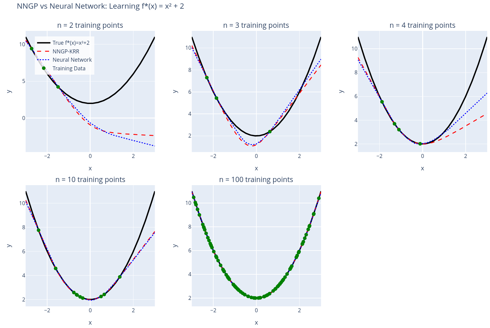
This is kinda ugly and IDK what to do with it. The limitations of kernels results should hold. I ran a few inductive bias experiments to compare the NNGP with KRR to NNs with AdamW but they are not that interesting and I think they were a waste of time (see the dropdown below).

Inductive bias experiment

Here's KRR with the one hidden layer ReLU NNGP and and train a one hidden layer ReLU NN to learn $f^{\ast }(x)=x^2+2$ with various numbers of training data points. All NNs trained to convergence. Weight decay in AdamW changes things, here I used 1e-6. Also, ${\sigma }_w={\sigma }_b=1$ .

Signal propagation

Deep signal propagation studies the statistics of hidden representation in deep NNs. They found some cool links to this work, most cleanly for tanh and also for ReLU.

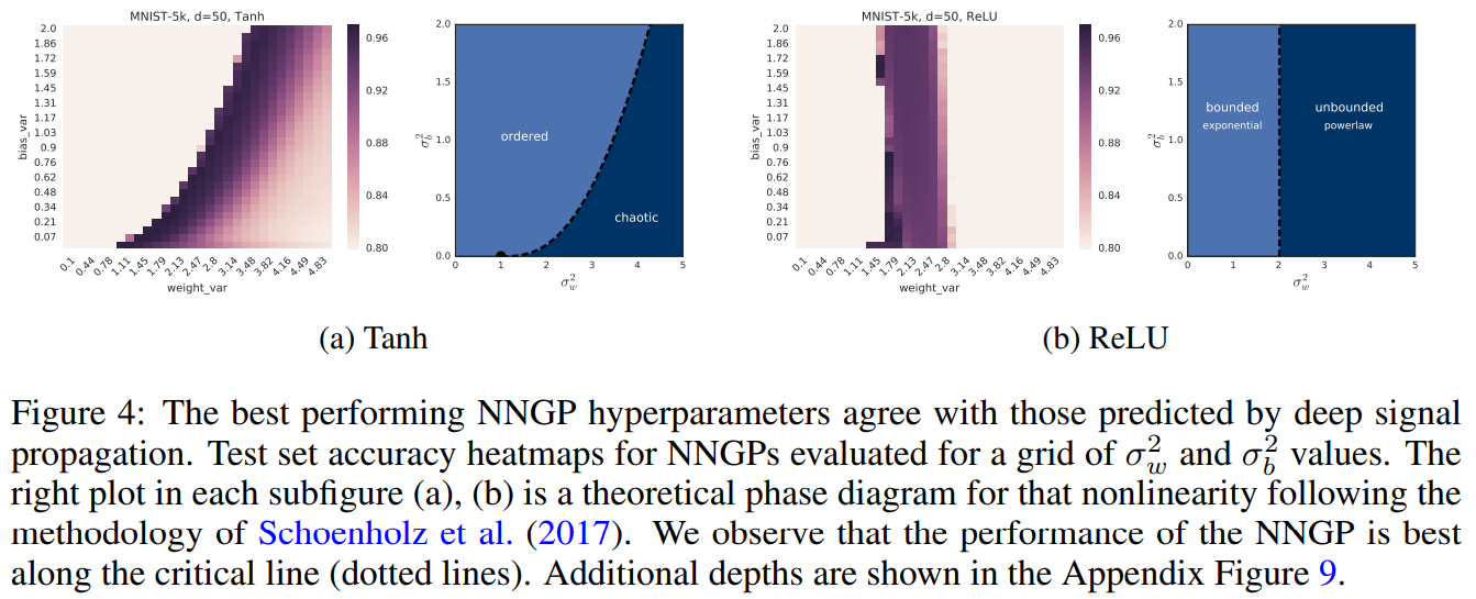
For tanh, the deep signal prop works identified an ordered and a chaotic phase, depending on $\sigma_w^2$ and $\sigma_b^2$. In the ordered phase, similar inputs to the NN yield similar outputs. This occurs when $\sigma_b^2$ dominates $\sigma_w^2$. In the NNGP, this manifests as $K^\infty (x, x')$ approaching a constant function. In the chaotic phase, similar inputs to the NN yield vastly different outputs. This occurs when $\sigma_w^2$ dominates $\sigma_b^2$. In the NNGP, this manifests as $K^\infty (x, x)$ approaching a constant function and $K^\infty (x, x')$ approaching a smaller constant function. In other words, in the chaotic phase, the diagonal of the kernel matrix is some value and off diagonals are all some other, smaller, value.

Interestingly, the NNGP performs best near the threshold between the chaotic and ordered phase. As depth increases, we converge towards $K^\infty (x, x')$, and only perform well closer and closer to the threshold. We do well at the threshold, because there, convergence to $K^\infty (x, x')$ is much slower (this is bc of some deep signal prop stuff I don’t understand).

Other experiments

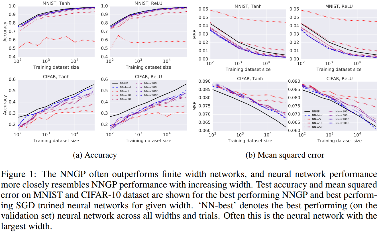
They ran experiments (Figure 1) that showed on MNIST and CIFAR-10 NNs and NNGP do essentially equally well. This indicates that feature learning is not important to do well on MNIST and CIFAR-10! (TODO: Find similar experiment on ImageNet and other datasets).

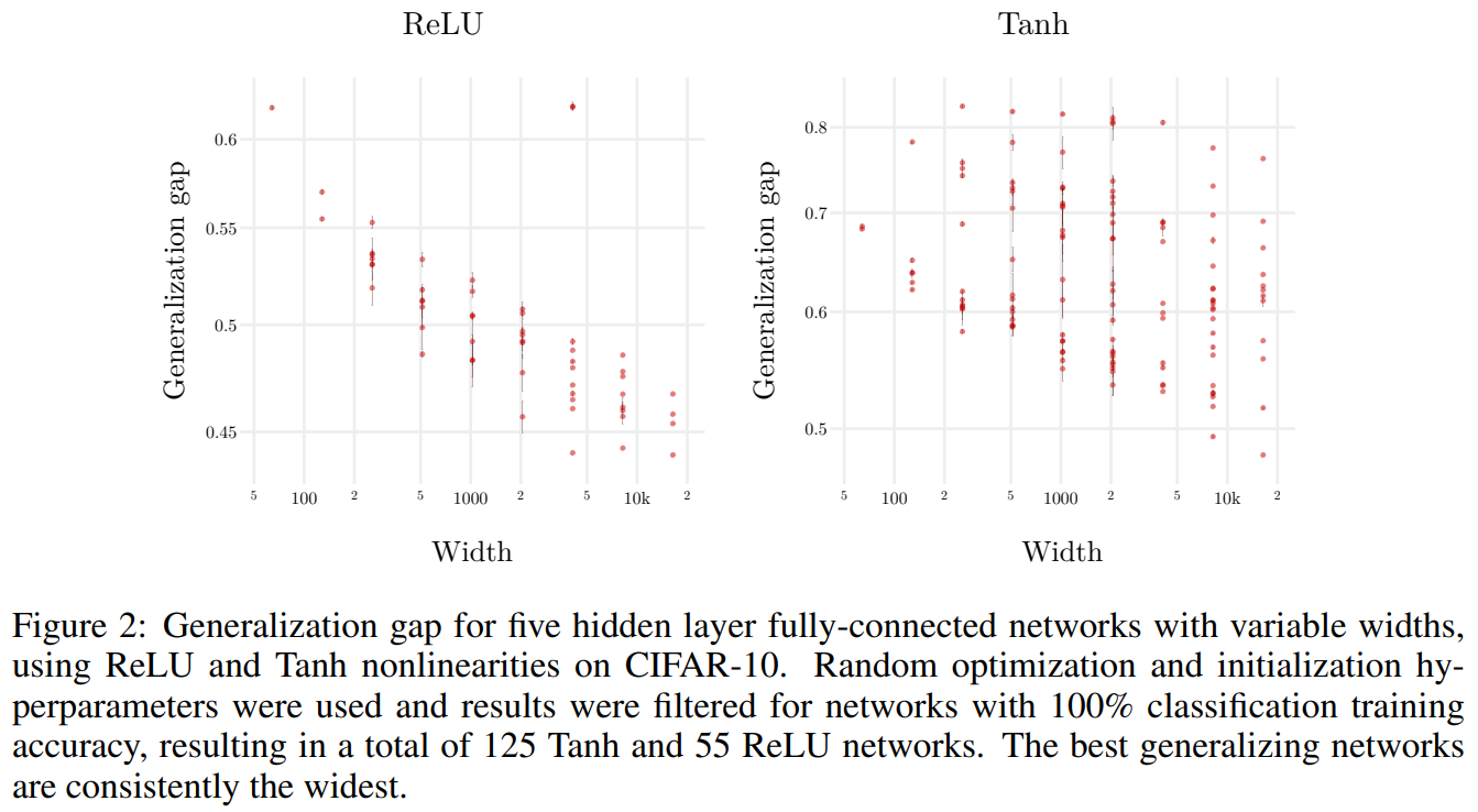
Additionally, they ran experiments (Figure 2) that showed increasing width improves generalization for fully connected MLPs on CIFAR-10. TODO: why I should expect this?

They also show that the NNGP uncertainty is well correlated with empirical error on MNIST and CIFAR. It’s nice that you get uncertainty estimates for free.

TODO: How computationally expensive is the NNGP?

TODO: How does the NNGP compare to the NTK, RBF, and other kernels?