A Gaussian process (GP) is a stochastic process (a collection of random variables indexed by time or space), such that every finite collection of those random variables has a multivariate normal distribution (copied from Wikipedia).

Some GPs (specifically stationary GPs, meaning it has a constant mean and covariance only depends on relative position of data points), have an explicit representation, where you can write it as

for some random variables $R$ and some fixed deterministic function $g$ (I think this is true).

Bayesian inference and prediction with a GP

We have a training set $\mathcal{D} = \{ (x^{(1)}, y^{(1)}), \ldots, (x^{(n)}, y^{(n)}) \}$, and we wish to make a Bayesian prediction (see my notes on Bayesian stuff for the difference between Bayesian inference and prediction) on a test sample $x$ using our GP, which is a distribution over functions.

We consider the following noise model, $y^{(i)} = g(x^{(i)}) + \epsilon^{(i)}$, where $\epsilon^{(i)} \sim \mathcal{N}(0, \sigma_n^2)$.

Our joint prior on labels is

From here, you just do the standard conditioning a joint Gaussian stuff (Wikipedia page for this). Then you can write this as a new GP. This is your posterior predictive.

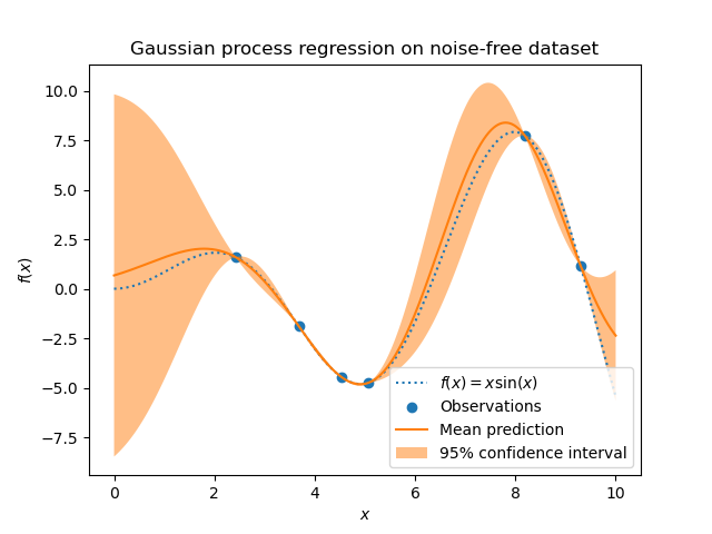
You can place a GP prior over functions and then compute the posterior after seeing data to have some probability distribution for what the rest of the functin looks like. This is what they call Gaussian process regression. They get these cool visualizations from it like this from on scikit-learn.

But also, the argmax sample from the posterior predictive corresponds to the kernel ridge regression solution,

where $\sigma_n^2$ is your ridge penalty / noise. This is just the mean solution in the plot above, so if you don’t care about the uncertainty quantification just do this ^.

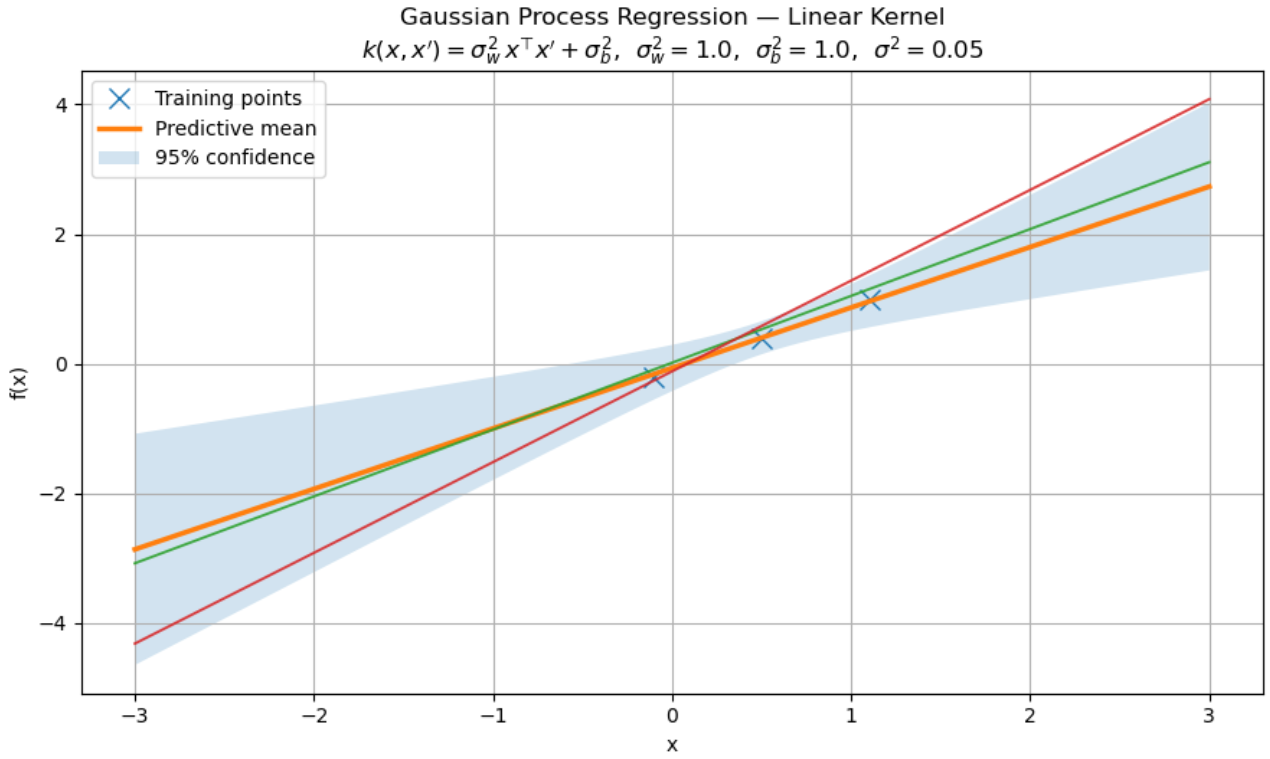
TODO: Maybe an example with a linear kernel?